
BOOM! A Mathematical Exploration of Big Waves and Sudden Bursts
Dynamical Systems and Bursting Phenomena | Cindy Wang
Bursts of activity are an interesting and important phenomenon in physical and biological systems. For example, rogue waves are large, unpredictable waves in the ocean. In other words, they are bursts in the amplitude of waves. Out of the many mechanisms that lead to rogue waves, one that does not assume energy in the ocean is constant is considered in this article. The waves are modelled by variables and by studying the equations that describe the rate of change of the variables, a possible reason for the burst is explained and confirmed using software.
Rogue waves are large, unpredictable waves in the ocean that are not associated with a storm system or tsunami. They are also known as freak waves, monster waves, episodic waves, killer waves, extreme waves, and abnormal waves. From these names it can be inferred that rogue waves may be extremely dangerous, especially to ships and isolated structures such as lighthouses. From an oceanographic point of view, rogue waves are usually defined as waves that exceed twice the significant wave height, which is itself defined as the mean of the largest third of waves that occur over a given period; rogue waves are extremely high compared to the waves surrounding it. While high waves are dangerous, what is more terrifying about rogue waves is their unpredictability. To try and understand when and how rogue waves occur, mathematical models can be applied.
Figure 2: Diagram of the three-dimensional state space with the infinite amplitude subspace and trajectory to indicate the mechanism of a burst. Produced in Microsoft Powerpoint.
The blue region is where r is finite, and the white region Σ represents where r tends to infinity (r —> ∞) or similarly, where r is much greater than one (r>>1). If a trajectory goes into, then comes out of Σ, then the amplitude would go to infinity and back, and that would be a burst. To understand when this would happen, the dynamics within ∑ were considered.
In a dynamical system, solutions to the equations equalling zero are also referred to as fixed points because at these points, the change of variables would be zero, so the variables will stay at the fixed point values. These fixed points might attract trajectories around it, repel trajectories, or attract in some directions and repel in the others. There are also periodic solutions where variables stay in the periodic pattern. For a burst to happen, there must exist two relevant solutions, B and A, which are fixed points or periodic solutions in ∑. At some finite amplitude state, the trajectory is close enough to the B solution to be attracted to it. There, the rate of change of r is so high (r tends to infinity) that the trajectory enters ∑. The solution B does not attract solutions in all directions, so the trajectory is sent away from B and is attracted by A. Then, as the trajectory nears A, A sends it away in the r direction and amplitude comes down and becomes finite. The trajectory therefore leaves ∑ and a burst occurs.
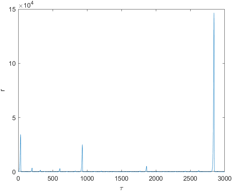
(a) y0=(10², 1.6, 0) and r in linear scale
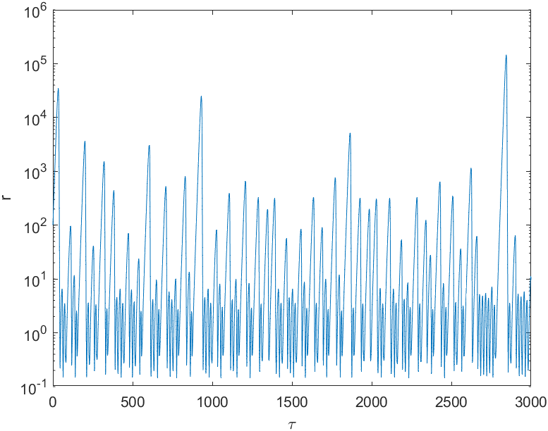
(b) y0=(10², 1.6, 0) and r in logarithmic scale
There are multiple mechanisms leading to rogue waves that are being studied. For example, small amplitude waves with different frequencies traveling in different directions that are superposed in the ocean could lead to rogue waves. Mechanisms that arise from physical factors, such as wave and current interactions or wind and pressure interactions, are also studied. Other well-studied mechanisms involve large amplitude nonlinear waves that are not perfectly sinusoidal [2-3]. However, these mechanisms assume that energy is constant, which is not the case in the ocean since the ocean interacts with other systems through channels such as sunlight, organic matter, and friction. Therefore, I considered a mechanism that does not make such an assumption in my summer research project.
There are multiple mechanisms leading to rogue waves that are being studied. For example, small amplitude waves with different frequencies traveling in different directions that are superposed in the ocean could lead to rogue waves. Mechanisms that arise from physical factors, such as wave and current interactions or wind and pressure interactions, are also studied. Other well-studied mechanisms involve large amplitude nonlinear waves that are not perfectly sinusoidal [2-3]. However, these mechanisms assume that energy is constant, which is not the case in the ocean since the ocean interacts with other systems through channels such as sunlight, organic matter, and friction. Therefore, I considered a mechanism that does not make such an assumption in my summer research project.
Model
This mechanism considers a container that is very close to a square. In the container, there are two waves travelling towards each other that are only slightly different. These waves interact and produce rogue waves. While this can be investigated experimentally, mathematics is used to model what happens to explore the mechanism more abstractly and precisely. Therefore, the mathematical representation of the ocean waves we investigate is referred to as the model.
In the model, the waves are described by a combination of four variables: r for the amplitude and ϑ, Φ ,Ψ each representing an angle. This is a use of Bloch Spherical Coordinates [4]. The motion or dynamics of the variables are described by the following equations [5]:

The left-hand side is notation for the rate of change (or the derivative of a function). The rate of change is of the variable on the top with respect to the variable on the bottom, which is time (τ) in this case. These equations form a dynamical system, because they are a set of equations that describe the rate at which variables change with respect to time. As in this case, the rate of change of certain variables often depends on other variables; the variables are “coupled”. This intertwined relationship means the equations are a system, hence the name dynamical systems.
In this model, rogue waves are represented by rogue bursts, which are large, unpredictable bursts in amplitude as shown later in Figure 3. The question to investigate, then, is “How does the model show bursts?”
Before the question is answered, a further look at the equations is necessary. Notice that Ψ does not appear in any of the first three equations, which means “decouples” from the rest of the equations. This means if the value of all the other variables do not depend on Ψ and if they are known, the value of Ψ can also be found from the last equation. So, to reduce workload, we focus on the first three equations, which form a three dimensional system. The corresponding state space is shown in Figure 2.
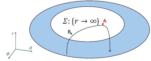
Figure 3: Amplitude r against time τ for varied initial conditions, r scalings y0=(r0, ϑ0, Φ0) near a B solution with parameter values: A=1—1.5i, B=—2.8+5i, C=1+1i, λ = 0.1, ∆λ=0.06, ∆ω =—0.01. Produced by ode23s in Matlab R2024b with default settings.
Bursts by Computation
For a set of parameter and initial condition values, we can use software to explore what happens as time goes on. The program considers the current state, then takes a step in state space based on the change of variables as dictated by the equations. The program is therefore referred to as a time-stepper. With consideration from previous literature [6], parameter values that are known to show large amplitude bursts were taken. Beginning near a B solution, bursts near the start of time are demonstrated as in Figure 3. After the trajectory eventually returns to a finite amplitude, it becomes close to another relevant B solution and other bursts occur.
Note that Figure 3(a) has r in linear scale to show simply how bursts compare with normal activity. However, linear scale only makes the biggest bursts visible, so logarithmic scale is also used. The bursts do not seem as apparent because each step up on the scale is a multiplication rather than an addition on the linear scale. Figure 3(a) and (b) are essentially the same graph with different scaling, but Figure 3(b) shows more information, especially bursts that are smaller in size.
These bursts seem to be irregular in both time and amplitude, which is the desired behaviour, but the irregularity means that the length of time for which we run the time-stepper might restrict us from seeing important dynamics. Notice that in Figure 3(b), the burst of the largest amplitude happens after when time τ is equal to 2,500. So, if we run the program for a shorter time period, this significant burst would not have been observed. A way to measure if the time-stepper has run for enough time is to see if the bursts in the second half of the total time are of a higher order of magnitude.
Through several comparisons, such as that of Figure 3(b) and 3(c), the computation suggests that the amplitude of the first burst is negatively correlated with the distance from the B solution in Σ. In other words, the closer we start to where trajectories push off to Σ, the closer we get to Σ before returning back to smaller amplitudes.
Discussion
In a mathematical sense, rogue waves do not only refer to those in the ocean, but also to similar activity in other systems. These rogue waves are also described as spatial-temporal bursts, since they are large bursts in amplitude that are unpredictable in space and time. However, in this model, only temporal bursts are explored. This is because the model only depends on time. The model makes the assumption that space is uniform, meaning the entire region acts as one. So, when rogue bursts are used to model rogue waves in the ocean, it would model the entire ocean to go up and then come back down again, which is clearly not the case. Further investigation has been done where there are a few of these models, each of which are an oscillator representing some region. Then, these oscillators are coupled together in a ring, so that they affect each other’s motion. Then, space is brought back into the system and will matter again [7].
Although the model is not perfect, it does provide a good basis for investigation into rogue waves and is also expected to be relevant to other applications with similar characteristics such as binary fluid convection (the transfer of heat in fluid), the Faraday system, nonlinear optics, and solar magnetic cycles.
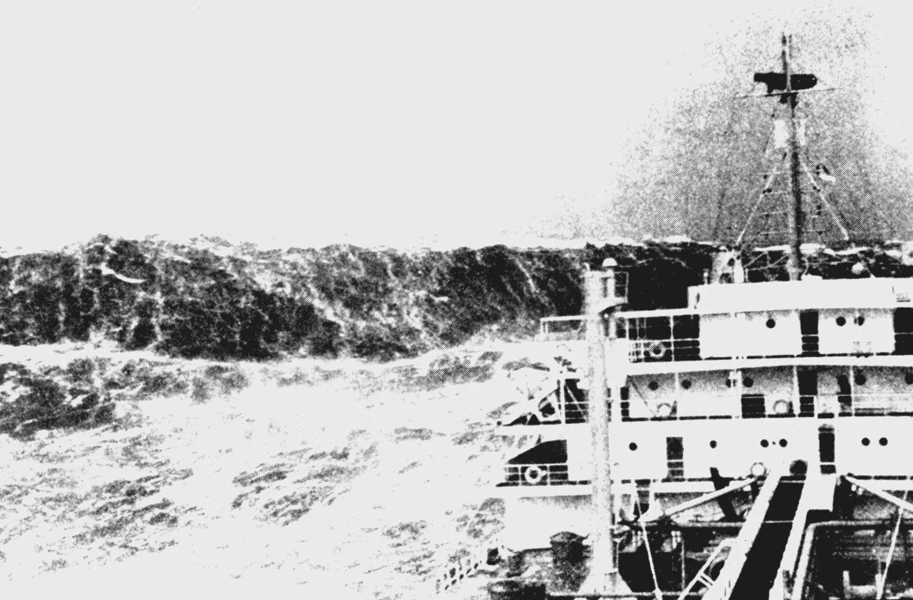
Figure 1: A rogue wave behind a merchant ship for scale.
Glossary
Initial Condition: The conditions posed by what value the variables take on at the start of time, when τ = 0.
Parameter: A quantity that defines certain characteristics of a system or function, influencing its behavior and outcomes. Unlike variables, which can change during the operation of a system, parameters remain constant within a specific context but can vary between different scenarios. In the system of equations, parameters include λ, ω, and AR .
State: The complete set of variables that describe the system at a given moment.
Superpose: The placement of one thing on or above another.
Trajectory: The path that a system’s state, in other words its variables, follows over time.

(c) y0=(105, 1.6, 0) and r in logarithmic scale
Acknowledgments
I would like to thank my supervisor, Dr. Priya Subramanian, for her support and guidance. Her understanding of the experience of being a beginner in research made my first research experience extra fulfilling. Her support extends beyond the project, including her encouragement and advice for this article. I also want to express my appreciation to the Department of Mathematics and fellow summer research students for the friendly academic environment.
[1] NOAA. wea00800: Merchant ship laboring in heavy seas as huge wave looms astern. Huge waves are common near the 100-fathom curve on the Bay of Biscay. (1993). [Online]. Available: https://www. flickr.com/photos/noaaphotolib/
[2] E. Pelinovsky and C. Kharif, Extreme Ocean Waves. Cham, Switzerland: Springer International Publishing, 2016.
[3] A. Osborne, Nonlinear Ocean Waves and the Inverse Scattering Transform, 1st ed. Amsterdam, Netherlands: Elsevier, 2010.
[4] F. Bloch, “Nuclear Induction,” Physical Review, vol. 70, no. 7–8, pp. 460–474, Oct. 1946, doi: https://doi.org/10.1103/physrev.70.460.
[5] J. Moehlis and E. Knobloch, “Bursts in oscillatory systems with broken D4 symmetry,” Physica D Nonlinear Phenomena, vol. 135, no. 3–4, pp. 263–304, Jan. 2000, doi: https://doi.org/10.1016/s0167- 2789(99)00141-4.
[6] E. Knobloch and J. Moehlis, “Burst mechanisms in hydrodynamics,” arXiv, 1999. [Online]. Available: https://arxiv.org/abs/physics/9909036.
[7] P. Subramanian, E. Knobloch, and P. G. Kevrekidis, “Forced symmetry breaking as a mechanism for rogue bursts in a dissipative nonlinear dynamical lattice,” Phys. Rev. E, vol. 106, no. 1, p. 014212, Jul. 2022, doi: https://doi.org/10.1103/PhysRevE.106.014212.

Cindy is in her third year of studying mathematics and will complete her honours next year. She is excited to continue her exploration in different fields of mathematics to find her interests and what she will focus on in the future